class: center, middle, inverse, title-slide .title[ # EDUC 847 Winter 24 ] .subtitle[ ## Week 6 - Logistic Regression ] .author[ ### Eric Brewe <br> Professor of Physics at Drexel University <br> ] .date[ ### 26 February 2024, last update: 2024-02-26 ] --- # Let's start with a complete dataset Start by getting the data into R ```r #This loads the csv and saves it as a dataframe titled sci_df sci_df <- read_csv(here("data", "sci_scores.csv")) ``` --- # Let's remember last class ### We predicted science scores from scores. ```r *sci_mod_motiv <- lm(sci ~ motiv, data = sci_df) tidy(summary(sci_mod_motiv)) ``` ``` ## # A tibble: 2 × 5 ## term estimate std.error statistic p.value ## <chr> <dbl> <dbl> <dbl> <dbl> ## 1 (Intercept) 405. 179. 2.26 0.0242 ## 2 motiv 5.46 2.42 2.25 0.0247 ``` Note - we have a new dataset, there is a passing variable. --- # Let's go futher ## What if we wanted to then predict who would pass some class. ### Probably need to look at our data ```r glimpse(sci_df) ``` ``` ## Rows: 500 ## Columns: 7 ## $ id <dbl> 23926, 31464, 42404, 19892, 76184, 58204, 38741, 72934, 11248,… ## $ gr <dbl> 4, 1, 2, 5, 3, 5, 2, 1, 1, 1, 2, 4, 2, 2, 1, 4, 5, 3, 4, 4, 3,… ## $ motiv <dbl> 80.88924, 62.60343, 85.45784, 102.34612, 97.08309, 69.99991, 5… ## $ pre_sc <dbl> 1.2129432, 1.2509983, 0.4046275, 2.6644015, 2.2353431, 0.15801… ## $ math_sc <dbl> 49.96987, 56.89187, 66.24704, 55.24663, 67.59779, 61.99406, 77… ## $ sci <dbl> 598.1784, 611.6507, 409.3981, 1185.3010, 1193.5658, 267.1035, … ## $ pass <dbl> 1, 0, 1, 1, 1, 1, 0, 1, 0, 1, 0, 0, 0, 0, 1, 1, 0, 1, 1, 1, 0,… ``` --- # Let's review passing data ```r sci_df %>% tabyl(pass) ``` ``` ## pass n percent ## 0 180 0.36 ## 1 320 0.64 ``` ### We need to be able to predict better than 64% --- # Let's plot ## We can try a scatter plot .pull-left[ ```r sci_df %>% ggplot(aes(x = motiv, y = pass)) + geom_point() ``` ] .pull-right[ 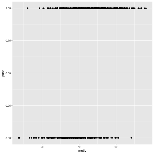<!-- --> ] --- # Let's plot ## Boxplots should be better .pull-left[ ```r sci_df %>% ggplot(aes(x = as.factor(pass), y = motiv)) + geom_boxplot() ``` ] .pull-right[ 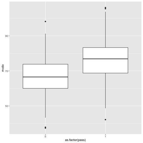<!-- --> ] --- # Let's predict passing ## Here's what we know: - Pass / Fail is a binary outcome variable - We have a variety of types of predictor variables ### Regular linear regression won't work. --- # Let's look at Logistic Regression .pull-left[ ## Goal of logistic regression is to predict a binary outcome * Linear regression - fit a slope to a data set. * Logistic regression - fit a logit to a data set. ] .pull-right[ 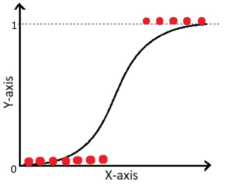 ] --- # Let's look at motivation .pull-left[ ```r sci_df %>% ggplot(aes(x = motiv, y = pass)) + geom_point() + geom_smooth(method = "glm", method.args = list(family = "binomial"), se = FALSE) ``` ] .pull-right[ 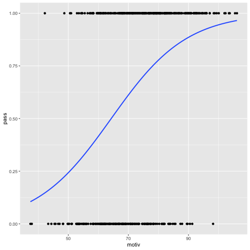<!-- --> ] --- # Let's do some math! ## The logistic funcion is: `\(\sigma(x) = \frac{1}{1+e^{-x}}\)` ### It has some important properties - it has a value between 0 and 1 for any value of x --- # Let's do some math! ## We can adapt this to a regression equation `\(p(x) = \frac{1}{1+e^{-(\beta_{0}+\beta_{1}x+...)}}\)` We interpret this as the probablility of the outcome variable, so in our case, it is the probability of passing. And by definition, the probability of failing the class is then `\(1 - p(x)\)` This means that the ratio of passing to failing is `\(\frac{p(x)}{1-p(x)} = e^{\beta_{0} + \beta_{1}x+...}\)` ### Why does this matter? We'll need to interpret the outcome of the regression. --- # Let's do logistic regression! ```r *pass_model <- glm(pass~motiv, data = sci_df, family = "binomial") summary(pass_model) ``` ``` ## ## Call: ## glm(formula = pass ~ motiv, family = "binomial", data = sci_df) ## ## Coefficients: ## Estimate Std. Error z value Pr(>|z|) ## (Intercept) -5.117806 0.695733 -7.356 1.9e-13 *** ## motiv 0.079602 0.009777 8.142 3.9e-16 *** ## --- ## Signif. codes: 0 '***' 0.001 '**' 0.01 '*' 0.05 '.' 0.1 ' ' 1 ## ## (Dispersion parameter for binomial family taken to be 1) ## ## Null deviance: 653.42 on 499 degrees of freedom ## Residual deviance: 568.99 on 498 degrees of freedom ## AIC: 572.99 ## ## Number of Fisher Scoring iterations: 4 ``` --- # Let's interpret ```r coef(pass_model) ``` ``` ## (Intercept) motiv ## -5.11780574 0.07960186 ``` But to interpret, we need to take the exp of the coefficient (because this is an log odds ratio) ```r exp(coef(pass_model)[2]) ``` ``` ## motiv ## 1.082856 ``` This means for every increase in motivation score, the odds of passing the class increase by ~8%. That seems meaningful. But how did we do? Is this better at predicting passing? --- # Let's evaluate ## A typical approach is to use a confusion matrix.  --- #Let's build a confusion matrix First, we will use the predict function to generate predicted probabilities of passing. ```r predicted <- tibble( probs = predict(pass_model, type = "response")) head(predicted) ``` ``` ## # A tibble: 6 × 1 ## probs ## <dbl> ## 1 0.789 ## 2 0.466 ## 3 0.844 ## 4 0.954 ## 5 0.932 ## 6 0.612 ``` But those are numbers, how do we convert to pass/fail? --- #Let's build a confusion matrix First, we will use the predict function to generate predicted probabilities of passing. ```r predicted %>% mutate(pred_50 = if_else(probs>0.5,1,0)) %>% mutate(pred_64 = if_else(probs>0.64,1,0)) -> predictions head(predictions, 10 ) ``` ``` ## # A tibble: 10 × 3 ## probs pred_50 pred_64 ## <dbl> <dbl> <dbl> ## 1 0.789 1 1 ## 2 0.466 0 0 ## 3 0.844 1 1 ## 4 0.954 1 1 ## 5 0.932 1 1 ## 6 0.612 1 0 ## 7 0.293 0 0 ## 8 0.831 1 1 ## 9 0.711 1 1 ## 10 0.287 0 0 ``` --- #Let's build a confusion matrix for the 50% ```r confusionMatrix(as.factor(sci_df$pass),as.factor(predictions$pred_50)) ``` ``` ## Confusion Matrix and Statistics ## ## Reference ## Prediction 0 1 ## 0 77 103 ## 1 49 271 ## ## Accuracy : 0.696 ## 95% CI : (0.6536, 0.7361) ## No Information Rate : 0.748 ## P-Value [Acc > NIR] : 0.9963 ## ## Kappa : 0.2939 ## ## Mcnemar's Test P-Value : 1.717e-05 ## ## Sensitivity : 0.6111 ## Specificity : 0.7246 ## Pos Pred Value : 0.4278 ## Neg Pred Value : 0.8469 ## Prevalence : 0.2520 ## Detection Rate : 0.1540 ## Detection Prevalence : 0.3600 ## Balanced Accuracy : 0.6679 ## ## 'Positive' Class : 0 ## ``` --- #Let's build a confusion matrix for the 64% ```r confusionMatrix(as.factor(sci_df$pass),as.factor(predictions$pred_64)) ``` ``` ## Confusion Matrix and Statistics ## ## Reference ## Prediction 0 1 ## 0 125 55 ## 1 107 213 ## ## Accuracy : 0.676 ## 95% CI : (0.633, 0.7169) ## No Information Rate : 0.536 ## P-Value [Acc > NIR] : 1.341e-10 ## ## Kappa : 0.3387 ## ## Mcnemar's Test P-Value : 6.151e-05 ## ## Sensitivity : 0.5388 ## Specificity : 0.7948 ## Pos Pred Value : 0.6944 ## Neg Pred Value : 0.6656 ## Prevalence : 0.4640 ## Detection Rate : 0.2500 ## Detection Prevalence : 0.3600 ## Balanced Accuracy : 0.6668 ## ## 'Positive' Class : 0 ## ``` --- # Let's define some terms **Sensitivity**: True Positive Rate - what percent of people did we predict would pass that actually did pass? **Specificity**: True Negative Rate - what percent of people did we predict would fail that actually did fail? **Precision**: Out of the people we predicted to pass, what percent actually did pass? **Recall**: Out of the people that did pass, what percent did we predict to pass? --- # Let's review We spent today looking at how to use logistic regression We can... - create a logistic regression model - interpret logistic regression coefficients - use a confusion matrix to evaluate the predictive power of the model