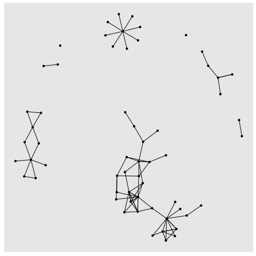
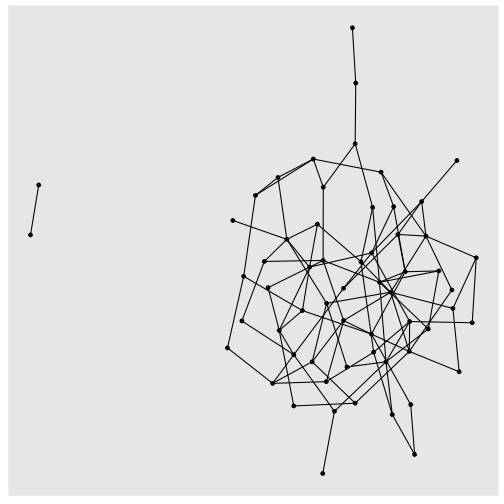
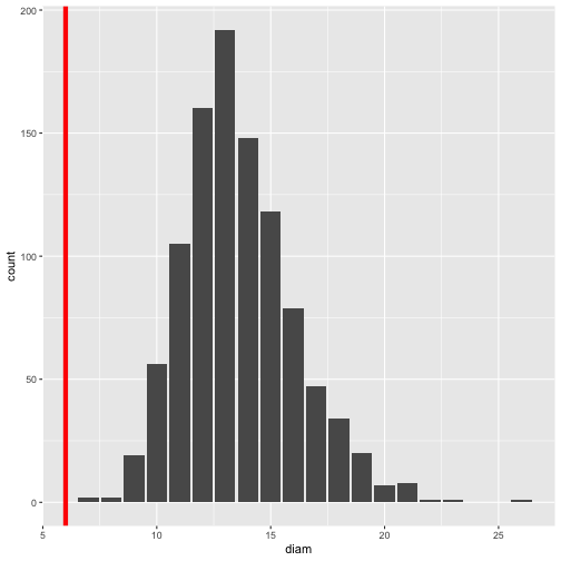
class: center, middle, inverse, title-slide .title[ # PEER Advanced Field School 2023 ] .subtitle[ ## Day 4 - Network Models ] .author[ ### Eric Brewe <br> Professor of Physics at Drexel University <br> ] .date[ ### 15 June 2023, last update: 2023-06-23 ] --- # Welcome Back! ### Our project is about building and analyzing the Workshop network We will continue to use the WorkshopNetwork.rds data file. ```r library(tidyverse) #tools for cleaning data library(igraph) #package for doing network analysis library(tidygraph) #tools for doing tidy networks library(here) #tools for project-based workflow library(ggraph) #plotting tools for networks library(boot) #to do resampling ``` --- # Let's load our data ```r gr <- readRDS(here("data", "WorkshopNetwork.rds")) ``` --- # Let's plot it quickly And get some important features of the graph. .pull-left[ ## Whare are distinctive features of the network? ```` ```r GrLayout <- create_layout(gr, layout = "kk") ggraph(GrLayout) + geom_edge_link() + geom_node_point() + theme(legend.position="bottom") ``` ```` ] .pull-right[ <!-- --> ] ```r gr ``` ``` ## # A tbl_graph: 60 nodes and 101 edges ## # ## # A directed multigraph with 8 components ## # ## # A tibble: 60 × 4 ## name AMPM Dessert Pages ## <chr> <chr> <chr> <dbl> ## 1 5106 morning person. Brownies 350 ## 2 6633 morning person. I don't care for dessert. 12 ## 3 7599 night owl. Ice Cream 300 ## 4 4425 morning person. I don't care for dessert. 0 ## 5 2495 morning person. Brownies 264 ## 6 6355 night owl. Ice Cream 4 ## # ℹ 54 more rows ## # ## # A tibble: 101 × 2 ## from to ## <int> <int> ## 1 1 1 ## 2 2 35 ## 3 3 14 ## # ℹ 98 more rows ``` Note, there are 60 nodes and 101 edges --- .center.font200[Orient] --- # Let's decide if our network is unique ### What is the big problem with the network that we have collected? -- 1. We have one network. 2. There is no variance in the metrics. 3. What is the null hypothesis/model? --- # Let's talk about camps ### This is a place where there are sort of two camps of network analysis .pull-left[ ### Statistical Camp - **Variance:** Permutation/resampling techniques such as bootstrap. - **Null hypothesis:** Exponential random graph models (ERGMs) Or rewired network ] .pull-right[ ### Graph Theoretic Camp - **Null Model** Theory driven models - Random Graph (Erdos-Renyi) - Small World (Watts-Strogatz) - Preferential Attachment (Barabasi-Albert) - **Variance** Network simulation ] --- # Let's compare two networks .pull-left[ ```r GrLayout <- create_layout(gr, layout = "kk") ggraph(GrLayout) + geom_edge_link() + geom_node_point() + theme(legend.position="bottom") ``` <!-- --> ] .pull-right[ ```r er_gr <- play_erdos_renyi(n = 60, m = 101, loops = FALSE) GrLayoutER <- create_layout(er_gr, layout = "kk") ggraph(GrLayoutER) + geom_edge_link() + geom_node_point() + theme(legend.position="bottom") ``` <!-- --> ] --- # Let's talk about how you might compare ### What are some ways you can think of to compare these two graphs? --- # Let's compare based on metrics Why don't we try density ```r edge_density(gr) ``` ``` ## [1] 0.02853107 ``` ```r edge_density(er_gr) ``` ``` ## [1] 0.02853107 ``` Well that isn't any fun! --- # Let's compare based on metrics Here is diameter, note that with tidygraph you have to use the with_graph() function, and specify the graph and function graph_diameter() ```r with_graph(gr, graph_diameter()) ``` ``` ## [1] 6 ``` ```r with_graph(er_gr, graph_diameter()) ``` ``` ## [1] 12 ``` Ok, so the numbers are different...does that mean the graphs are different? --- # Let's try this 1000 times ```r #Start by setting up a vector to hold our results. diameter_results <- c() for(i in 1:1000) { tmp <- play_erdos_renyi(n=60, m = 101) diameter_results[i] = with_graph(tmp, graph_diameter()) } #Convert to dataframe diameter_results_df <- tibble(diam = diameter_results) #and plot our results ggplot(diameter_results_df, aes(diam)) + geom_bar() + geom_vline(xintercept = with_graph(gr, graph_diameter()), color = 'red', size = 2) ``` <!-- --> --- # Let's get a confidcence interval ### If we want to estimate the confidence with which we think our measured network is different on any metrics, we can look for the percentiles. Let's see if the measured diameter falls within the 95% of the simulated network.... ```r mean(diameter_results_df$diam) ``` ``` ## [1] 13.608 ``` ```r sd(diameter_results_df$diam) ``` ``` ## [1] 2.450376 ``` ```r quantile(diameter_results_df$diam, probs = c(0.025, 0.975)) ``` ``` ## 2.5% 97.5% ## 10 19 ``` Since the measured diameter of 6 is outside of this range, we can say pretty confidently that the measured network is not a random network! --- # Let's summarize .font160[ 1. We measured one network 2. To compare we generated a network (in this case it was random) 3. We replicated 1000 times 4. We checked whether metrics from the measured network falls within some confidence range. 5. We can say the measured network is different than random. ] --- # Let's assign attributes ### In order to compare homophily, we need our ER_gr to have the same attributes. There is a file that has a random graph with the attributes assigned to it. ```r ER_gr_attr <- readRDS(here("data", "RandomGraph.rds")) ``` ``` ## # A tbl_graph: 58 nodes and 101 edges ## # ## # A directed simple graph with 1 component ## # ## # A tibble: 58 × 3 ## name AMPM Dessert ## <chr> <chr> <chr> ## 1 5106 morning person. Brownies ## 2 6633 morning person. I don't care for dessert. ## 3 7599 night owl. Ice Cream ## 4 4425 morning person. I don't care for dessert. ## 5 2495 morning person. Brownies ## 6 6355 night owl. Ice Cream ## # ℹ 52 more rows ## # ## # A tibble: 101 × 2 ## from to ## <int> <int> ## 1 1 12 ## 2 1 25 ## 3 1 33 ## # ℹ 98 more rows ``` ### Now you get to try! - Choose a network simulator (think about why you chose it) - Decide on a metric (better yet - create a function to look at many at once). - Simulate networks -- Measure chosen metrics -- Store metrics in data frame --- # Let's reflect .font120[ We did it! 1. We can import data into R 2. We can manipulate these data 3. We can create a network 4. We can plot a network 5. We can calculate a number of centrality measures 6. We can use these in plotting networks 7. We can use these in testing hypotheses 8. We can calculate a number of whole graph metrics 9. We can use these in comparing networks ] --- # Let's note what we missed .font150[ 1. We didn't really touch Base R 2. We didn't deal with ERGMs. ] --- # Let's be thankful .font200.center[ Thanks to PEER Thanks to all of you 👏 ]