EDUC 847 Winter 25
Week 2 - Fundamentals of Linear Modeling
Eric Brewe 
 Professor of Physics at Drexel University 

15 January 2025, last update: 2025-01-18
1 / 17

Let's start where we ended last class...Scatter Plots

Start by getting the data into R

#This loads the csv and saves it as a dataframe titled week_1_data
week_1_data <- read_csv(here("static/slides/EDUC_847/data",
                             "EDUC_847_Survey.csv"))

2 / 17

Let's start cleaning up.

First, we don't need most of that data

There is a ton of data there that doesn't make sense for us to keep around.

We will use the '%>%' (pipe) operator and the verb select

week_1_data %>%
  select(ID,Q2:Q6) -> w1df
glimpse(w1df)

## Rows: 10
## Columns: 6
## $ ID <dbl> 523, 876, 490, 166, 318, 626, 655, 182, 219, 305
## $ Q2 <chr> "I am more of a", "{\"ImportId\":\"QID4\"}", NA, "1", "2", "1", "1"…
## $ Q3 <chr> "My favorite dessert is", "{\"ImportId\":\"QID2\"}", NA, "1", "1", …
## $ Q4 <chr> "Which of the following beverages have you had this week (select al…
## $ Q5 <chr> "How many pages were in the book that is physically closest to you?…
## $ Q6 <chr> "Estimate the weight of this cow. Please enter a number.", "{\"Impo…

3 / 17

Let's keep cleaning up.

Notice there are two rows of data that are just the questions and something from Qualtrics. Let's get rid of those.

w1df %>%
  filter(row_number() >3 ) -> w1df

4 / 17

Let's lump all this together so we don't have to do it again.

week_1_data %>%
  select(ID,Q2:Q6) %>%
  filter(row_number() >3 ) %>%
  mutate(across(c(Q2:Q3,Q5:Q6), as.numeric)) -> w1df

5 / 17

Let's look at books vs. weight of cow

Is there a relationship between length of book (Q5) and estimates on weight of cow (Q6)?

Making a scatter plot to explore

w1df %>%
  select(Q5:Q6) %>%
  ggplot(aes(x = Q5, y = Q6)) +
  geom_point() + 
  theme_minimal() + 
  labs(x = "Pages", 
       y = "Weight of Cow",
       title = "Kick Ass Scatterplot!")

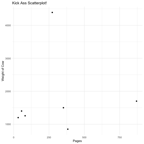
A residual is the distance between the Y value for each measurement, and the predicted Y value.

6 / 17

Let's investigate the residuals for our data

w1df %>% 
  select(Q5,Q6)

## # A tibble: 7 × 2
##      Q5    Q6
##   <dbl> <dbl>
## 1   273  4389
## 2    32  1200
## 3   383   850
## 4   352  1500
## 5   869  1700
## 6    56  1400
## 7    81  1256

7 / 17

Let's make a linear regression model

We want the estimated weight of the cow (Q6) as predicted by the length of the book closest to the survey respondent (Q5).

Model1 <- lm(Q6 ~ Q5, data = w1df)
Model1

## 
## Call:
## lm(formula = Q6 ~ Q5, data = w1df)
## 
## Coefficients:
## (Intercept)           Q5  
##   1668.7235       0.3001

8 / 17

Let's clean up our language...

In this situation, Q6 (the Estimated weight of the cow) is the Outcome Variable and Q5 (the number of pages in the closest book) is the Predictor variable.

Outcome Variable is often referred to as independent variable

Predictor Variable is often referred to as the dependent variable.

I hate this language. Predictor and Outcome are much more descriptive.

9 / 17

Let's figure out what this means

Model1

## 
## Call:
## lm(formula = Q6 ~ Q5, data = w1df)
## 
## Coefficients:
## (Intercept)           Q5  
##   1668.7235       0.3001

Intercept = if the closest book had 0 pages in it, this would be the estimated weight of the cow that we predict.

Q6 coefficient = If we increase the number of pages in the book, the value of the coeffient tells us how much we would increase the estimated weight of the cow by

10 / 17

Let's check out those residuals...

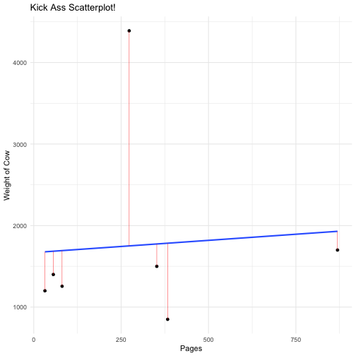
augment(Model1) %>%
  select(Q5:.resid)

## # A tibble: 7 × 3
##      Q5 .fitted .resid
##   <dbl>   <dbl>  <dbl>
## 1   273   1751.  2638.
## 2    32   1678.  -478.
## 3   383   1784.  -934.
## 4   352   1774.  -274.
## 5   869   1929.  -229.
## 6    56   1686.  -286.
## 7    81   1693.  -437.

11 / 17

Let's see how much better the model fits

augment(Model1) %>%
  select(Q5:.resid) %>%
  mutate(SqResid = .resid^2)

## # A tibble: 7 × 4
##      Q5 .fitted .resid  SqResid
##   <dbl>   <dbl>  <dbl>    <dbl>
## 1   273   1751.  2638. 6960935.
## 2    32   1678.  -478.  228795.
## 3   383   1784.  -934.  871700.
## 4   352   1774.  -274.   75266.
## 5   869   1929.  -229.   52662.
## 6    56   1686.  -286.   81526.
## 7    81   1693.  -437.  190994.

12 / 17

Let's see how much better the model fits

augment(Model1) %>%
  select(Q5:.resid) %>%
  mutate(SqResid = .resid^2) %>%
  tally(SqResid)

## # A tibble: 1 × 1
##          n
##      <dbl>
## 1 8461878.

13 / 17

Let's take a look at R²

R² is the measure of how well the model fits

$R^{2} = 1 - \frac{\sum_{i} (Y_{P r e d} - Y_{i})^{2}}{\sum_{i} (Y_{i} - \bar{Y})^{2}}$

augment(Model1) %>%
  select(Q6:.resid) %>%
  mutate(SqResid = .resid^2) %>%
  mutate(SqDiffMean = (Q6 - mean(Q6))^2) -> resid_df
glimpse(resid_df)

## Rows: 7
## Columns: 6
## $ Q6         <dbl> 4389, 1200, 850, 1500, 1700, 1400, 1256
## $ Q5         <dbl> 273, 32, 383, 352, 869, 56, 81
## $ .fitted    <dbl> 1750.642, 1678.326, 1783.649, 1774.347, 1929.481, 1685.527,…
## $ .resid     <dbl> 2638.3584, -478.3256, -933.6489, -274.3468, -229.4810, -285…
## $ SqResid    <dbl> 6960935.14, 228795.43, 871700.18, 75266.17, 52661.52, 81525…
## $ SqDiffMean <dbl> 6930432.327, 309612.755, 821612.755, 65755.612, 3184.184, 1…

14 / 17

Let's take a look at R²

$R^{2} = 1 - \frac{\sum_{i} (Y_{P r e d} - Y_{i})^{2}}{\sum_{i} (Y_{i} - \bar{Y})^{2}}$

SquaredResiduals = sum(resid_df$SqResid)
SquaredResiduals

## [1] 8461878

SquaredDiffMean = sum(resid_df$SqDiffMean)
SquaredDiffMean

## [1] 8508068

r2 = 1-(SquaredResiduals/SquaredDiffMean)
r2

## [1] 0.005428873

15 / 17

Let's compare to the R^2<\sup>

SquaredResiduals

## [1] 8461878

SquaredDiffMean

## [1] 8508068

r2

## [1] 0.005428873

summary(Model1)

## 
## Call:
## lm(formula = Q6 ~ Q5, data = w1df)
## 
## Residuals:
##      1      2      3      4      5      6      7 
## 2638.4 -478.3 -933.6 -274.3 -229.5 -285.5 -437.0 
## 
## Coefficients:
##              Estimate Std. Error t value Pr(>|t|)  
## (Intercept) 1668.7235   723.6088   2.306   0.0692 .
## Q5             0.3001     1.8163   0.165   0.8753  
## ---
## Signif. codes:  0 '***' 0.001 '**' 0.01 '*' 0.05 '.' 0.1 ' ' 1
## 
## Residual standard error: 1301 on 5 degrees of freedom
## Multiple R-squared:  0.005429,    Adjusted R-squared:  -0.1935 
## F-statistic: 0.02729 on 1 and 5 DF,  p-value: 0.8753

16 / 17

Let's recap

We can...

Fit a regression model to two continuous variables
Calculate the residuals
Calculate the squared residuals
Use the residuals to calculate the R²

17 / 17

Help

Keyboard shortcuts

↑, ←, Pg Up, k

Go to previous slide

↓, →, Pg Dn, Space, j

Go to next slide

Home

Go to first slide

End

Go to last slide

Number + Return

Go to specific slide

b / m / f

Toggle blackout / mirrored / fullscreen mode

Clone slideshow

Toggle presenter mode

Restart the presentation timer

?, h

Toggle this help

EDUC 847 Winter 25

Week 2 - Fundamentals of Linear Modeling

Eric Brewe Professor of Physics at Drexel University

15 January 2025, last update: 2025-01-18

Let's start where we ended last class...Scatter Plots

Let's start cleaning up.

First, we don't need most of that data

Let's keep cleaning up.

Let's lump all this together so we don't have to do it again.

Let's look at books vs. weight of cow

Is there a relationship between length of book (Q5) and estimates on weight of cow (Q6)?

Making a scatter plot to explore

Let's investigate the residuals for our data

Let's make a linear regression model

We want the estimated weight of the cow (Q6) as predicted by the length of the book closest to the survey respondent (Q5).

Let's clean up our language...

Let's figure out what this means

Let's check out those residuals...

Let's see how much better the model fits

Let's see how much better the model fits

Let's take a look at R2

Let's take a look at R2

Let's compare to the R2<\sup>

Let's recap

Let's start where we ended last class...Scatter Plots

Help

Eric Brewe
Professor of Physics at Drexel University

Let's take a look at R²

Let's take a look at R²

Let's compare to the R^2<\sup>