EDUC 847 Winter 24
Week 5 - Multiple Regression
Eric Brewe 
 Professor of Physics at Drexel University 

5 February 2025, last update: 2025-02-05
1 / 27

Let's start with a complete dataset

Start by getting the data into R

#This loads the csv and saves it as a dataframe titled week_1_data
sci_df <- read_csv(here("data",
                        "science_scores.csv"))

2 / 27

Let's remember last week

We want to predict a science score from a math score.

sci_mod_math <- lm(sci ~ math_sc, data = sci_df)
tidy(summary(sci_mod_math))

## # A tibble: 2 × 5
##   term        estimate std.error statistic    p.value
##   <chr>          <dbl>     <dbl>     <dbl>      <dbl>
## 1 (Intercept)     43.6    164.       0.265 0.791     
## 2 math_sc         11.6      2.47     4.70  0.00000343

Note - we have a new dataset, nothing is missing!

3 / 27

Let's use motivation in a model

sci_mod_motiv <- lm(sci ~ motiv, data = sci_df)
tidy(sci_mod_motiv)

## # A tibble: 2 × 5
##   term        estimate std.error statistic p.value
##   <chr>          <dbl>     <dbl>     <dbl>   <dbl>
## 1 (Intercept)   405.      179.        2.26  0.0242
## 2 motiv           5.46      2.42      2.25  0.0247

4 / 27

Let's reflect

tidy(sci_mod_math)

## # A tibble: 2 × 5
##   term        estimate std.error statistic    p.value
##   <chr>          <dbl>     <dbl>     <dbl>      <dbl>
## 1 (Intercept)     43.6    164.       0.265 0.791     
## 2 math_sc         11.6      2.47     4.70  0.00000343

tidy(sci_mod_motiv)

## # A tibble: 2 × 5
##   term        estimate std.error statistic p.value
##   <chr>          <dbl>     <dbl>     <dbl>   <dbl>
## 1 (Intercept)   405.      179.        2.26  0.0242
## 2 motiv           5.46      2.42      2.25  0.0247

5 / 27

Let's reflect

We have two models that predict science score.

Which is right?

Which is better?

6 / 27

Let's try something new

What if we put them both in the model?

sci_mod_motiv_math <- lm(sci ~ math_sc + motiv, data = sci_df)
tidy(sci_mod_motiv_math)

## # A tibble: 3 × 5
##   term        estimate std.error statistic     p.value
##   <chr>          <dbl>     <dbl>     <dbl>       <dbl>
## 1 (Intercept)  -473.      249.       -1.90 0.0581     
## 2 math_sc        12.2       2.47      4.96 0.000000981
## 3 motiv           6.53      2.38      2.75 0.00624

7 / 27

Let's interpret

## 
## Call:
## lm(formula = sci ~ math_sc + motiv, data = sci_df)
## 
## Residuals:
##    Min     1Q Median     3Q    Max 
## -855.8 -385.2 -183.7  139.6 4380.2 
## 
## Coefficients:
##             Estimate Std. Error t value Pr(>|t|)    
## (Intercept) -473.410    249.288  -1.899  0.05814 .  
## math_sc       12.239      2.469   4.957 9.81e-07 ***
## motiv          6.532      2.378   2.747  0.00624 ** 
## ---
## Signif. codes:  0 '***' 0.001 '**' 0.01 '*' 0.05 '.' 0.1 ' ' 1
## 
## Residual standard error: 648.8 on 497 degrees of freedom
## Multiple R-squared:  0.05673,    Adjusted R-squared:  0.05293 
## F-statistic: 14.95 on 2 and 497 DF,  p-value: 4.978e-07

8 / 27

Let's interpret graphically

avPlots(sci_mod_motiv_math)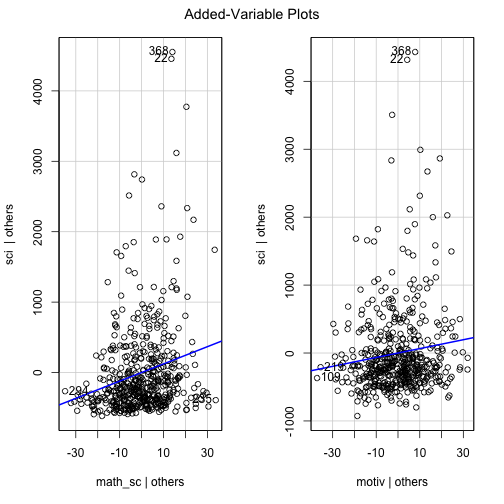

9 / 27

Let's look at these coefficients

plot_summs(sci_mod_motiv_math)

10 / 27

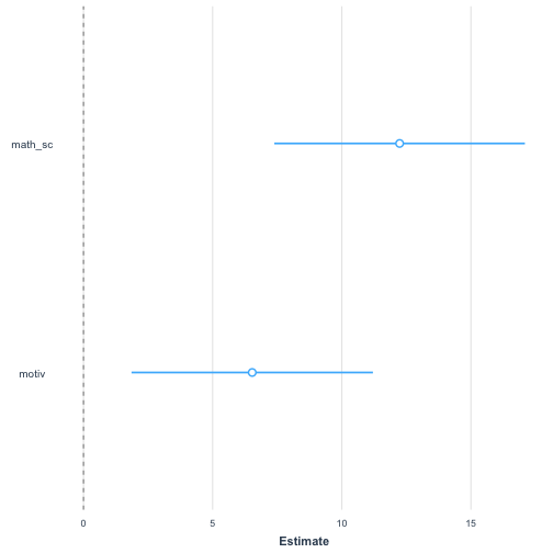
Let's look at these coefficients

plot_summs(sci_mod_motiv_math, inner_ci_level = 0.9)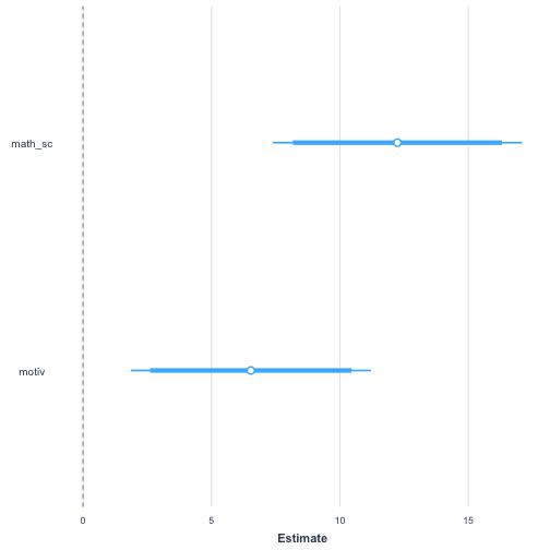

11 / 27

Let's review the goodness of fit

glance(sci_mod_motiv_math)

## # A tibble: 1 × 12
##   r.squared adj.r.squared sigma statistic     p.value    df logLik   AIC   BIC
##       <dbl>         <dbl> <dbl>     <dbl>       <dbl> <dbl>  <dbl> <dbl> <dbl>
## 1    0.0567        0.0529  649.      14.9 0.000000498     2 -3946. 7899. 7916.
## # ℹ 3 more variables: deviance <dbl>, df.residual <int>, nobs <int>

This give us some numbers, but we need to know what these mean.

12 / 27

Let's decide, is it a better model?

We have a few options...

Look at the $R^{2}$
Look at the adjusted $R^{2}$
- adj $R^{2} = 1 - \frac{S S_{r e s}}{S S_{t o t}} * \frac{N - 1}{N - K - 1}$
Akaike information criteria
- $A I C = \frac{S S_{r e s}}{σ} + 2 K$
- ==Lower is better!==
- to access AIC can use the step function in the emdi package

13 / 27

Let's look at AIC

To do this, we start with the full model and remove variables and recalculate the AIC. This is called backward selection.

step(sci_mod_motiv_math, 
     direction = "backward")

14 / 27

Let's look at AIC

## Start:  AIC=6478.14
## sci ~ math_sc + motiv
## 
##           Df Sum of Sq       RSS    AIC
## <none>                 209217142 6478.1
## - motiv    1   3175469 212392611 6483.7
## - math_sc  1  10345702 219562843 6500.3

## 
## Call:
## lm(formula = sci ~ math_sc + motiv, data = sci_df)
## 
## Coefficients:
## (Intercept)      math_sc        motiv  
##    -473.410       12.239        6.532

15 / 27

Let's compare models graphically

plot_summs(sci_mod_motiv, sci_mod_motiv_math, inner_ci_level = 0.9)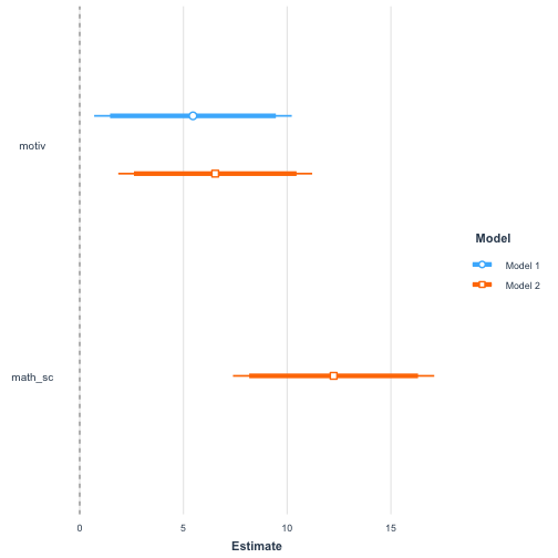

16 / 27

Let's compare statistically

We saw that the AIC went down, but more complicated models are typically worse (prone to overfitting, harder to interpret, etc...) Is there a way to compare the models statistically so we can decide if it is worth it to use the more complicated model. We will compare with an ANOVA

We will compare the model with the motivation score as compared to the model with just the math score.

anova(sci_mod_math, sci_mod_motiv_math)

## Analysis of Variance Table
## 
## Model 1: sci ~ math_sc
## Model 2: sci ~ math_sc + motiv
##   Res.Df       RSS Df Sum of Sq      F   Pr(>F)   
## 1    498 212392611                                
## 2    497 209217142  1   3175469 7.5434 0.006242 **
## ---
## Signif. codes:  0 '***' 0.001 '**' 0.01 '*' 0.05 '.' 0.1 ' ' 1

17 / 27

Let's try more variables

What about the group variable? Maybe some groups differ on math, motivation, and science score...

sci_mod_motiv_math_gr <- lm(sci~ math_sc + motiv + gr , data = sci_df)
tidy(sci_mod_motiv_math_gr)

## # A tibble: 4 × 5
##   term        estimate std.error statistic     p.value
##   <chr>          <dbl>     <dbl>     <dbl>       <dbl>
## 1 (Intercept)  -580.      257.       -2.25 0.0247     
## 2 math_sc        12.4       2.47      5.02 0.000000731
## 3 motiv           6.50      2.37      2.74 0.00639    
## 4 gr             33.3      20.6       1.62 0.106

18 / 27

Let's try more variables

What about the group variable? Maybe some groups differ on math, motivation, and science score...

plot_summs(sci_mod_motiv, 
           sci_mod_motiv_math, 
           sci_mod_motiv_math_gr, inner_ci_level = 0.9)

19 / 27

Let's dummy code

So, the main idea here is that we can see that group might matter...but we don't know which group. So let's set up separate variables for each group.

sci_df %>%
  mutate(Gr1 = case_when(gr == 1 ~ 1, 
                         gr != 1 ~0))  %>%
  head(., 20)

## # A tibble: 20 × 7
##       id    gr motiv pre_sc math_sc   sci   Gr1
##    <dbl> <dbl> <dbl>  <dbl>   <dbl> <dbl> <dbl>
##  1 23926     4  80.9  1.21     50.0  598.     0
##  2 31464     1  62.6  1.25     56.9  612.     1
##  3 42404     2  85.5  0.405    66.2  409.     0
##  4 19892     5 102.   2.66     55.2 1185.     0
##  5 76184     3  97.1  2.24     67.6 1194.     0
##  6 58204     5  70.0  0.158    62.0  267.     0
##  7 38741     2  53.2  0.168    77.6  234.     0
##  8 72934     1  84.3  0.130    72.4  307.     1
##  9 11248     1  75.6  0.415    74.7  406.     1
## 10 80068     1  52.9  5.50     73.7 2583.     1
## 11 17435     2  62.0  0.615    69.2  440.     0
## 12 72685     4  49.8  0.639    67.7  401.     0
## 13 91175     2  69.1  0.225    65.0  286.     0
## 14 30104     2  52.7  1.74     57.8  758.     0
## 15 20732     1  93.1  1.05     54.5  615.     1
## 16 55484     4  79.6  3.73     69.3 1786.     0
## 17 17753     5  62.1  0.715    54.5  415.     0
## 18 99371     3  48.7  1.55     48.7  587.     0
## 19 87933     4  74.8  0.122    85.6  281.     0
## 20 96189     4  82.7  0.346    66.6  381.     0

20 / 27

Let's dummy code

Now extend out to all groups and assign to new dataframe

sci_df %>%
  mutate(Gr1 = case_when(gr == 1 ~ 1, 
                         gr != 1 ~0))  %>%
  mutate(Gr2 = case_when(gr == 2 ~ 1, 
                         gr != 2 ~0)) %>%
  mutate(Gr3 = case_when(gr == 3 ~ 1, 
                         gr != 3 ~0)) %>%
  mutate(Gr4 = case_when(gr == 4 ~ 1, 
                         gr != 4 ~0)) %>%
  mutate(Gr5 = case_when(gr == 5 ~ 1, 
                         gr != 5 ~0)) -> sci_df_groups

21 / 27

Let's include the groups in a model

Need to use the new dataframe and add all the different groups

sci_mod_motiv_math_groups <- lm(sci~ math_sc + 
                                     motiv + 
                                     Gr1 +
                                     Gr2 +
                                     Gr3 +
                                     Gr4 +
                                     Gr5 , data = sci_df_groups)

22 / 27

Let's include the groups in a model

summary(sci_mod_motiv_math_groups)

## 
## Call:
## lm(formula = sci ~ math_sc + motiv + Gr1 + Gr2 + Gr3 + Gr4 + 
##     Gr5, data = sci_df_groups)
## 
## Residuals:
##    Min     1Q Median     3Q    Max 
## -912.0 -367.6 -171.8  143.9 4272.2 
## 
## Coefficients: (1 not defined because of singularities)
##             Estimate Std. Error t value Pr(>|t|)    
## (Intercept) -483.123    258.234  -1.871  0.06195 .  
## math_sc       12.325      2.470   4.989 8.42e-07 ***
## motiv          6.649      2.374   2.800  0.00531 ** 
## Gr1         -124.619     92.486  -1.347  0.17846    
## Gr2          -37.089     92.746  -0.400  0.68940    
## Gr3          101.630     93.212   1.090  0.27611    
## Gr4           38.948     91.611   0.425  0.67092    
## Gr5               NA         NA      NA       NA    
## ---
## Signif. codes:  0 '***' 0.001 '**' 0.01 '*' 0.05 '.' 0.1 ' ' 1
## 
## Residual standard error: 647 on 493 degrees of freedom
## Multiple R-squared:  0.06966,    Adjusted R-squared:  0.05834 
## F-statistic: 6.152 on 6 and 493 DF,  p-value: 3.096e-06

23 / 27

Let's explore interactions

What if a student's motivation is somehow connected to their math score?

We should look for interactions...

sci_mod_motiv_math_interactions <- lm(sci~ math_sc*motiv , data = sci_df)
summary(sci_mod_motiv_math_interactions)

## 
## Call:
## lm(formula = sci ~ math_sc * motiv, data = sci_df)
## 
## Residuals:
##    Min     1Q Median     3Q    Max 
## -889.1 -382.3 -174.8  127.0 4361.5 
## 
## Coefficients:
##               Estimate Std. Error t value Pr(>|t|)
## (Intercept)   277.5601   930.8814   0.298    0.766
## math_sc         0.6281    14.0845   0.045    0.964
## motiv          -3.8214    12.5920  -0.303    0.762
## math_sc:motiv   0.1605     0.1917   0.837    0.403
## 
## Residual standard error: 649 on 496 degrees of freedom
## Multiple R-squared:  0.05806,    Adjusted R-squared:  0.05236 
## F-statistic: 10.19 on 3 and 496 DF,  p-value: 1.597e-06

24 / 27

Let's plot this...

There are two ways, first, we can plot out the coefficients like we have done before...

plot_summs(sci_mod_motiv_math_interactions, inner_ci_level = 0.9)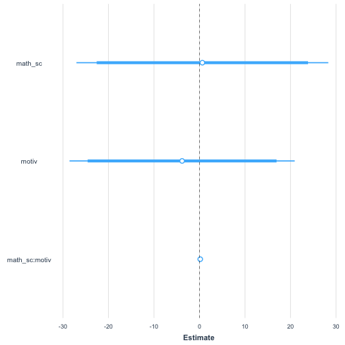

25 / 27

Let's plot this...

There are two ways, or we can use the interact_plot

interact_plot(model = sci_mod_motiv_math_interactions, pred =  math_sc, modx = motiv)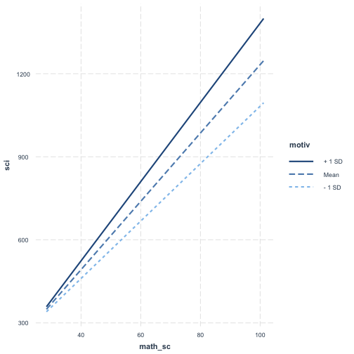

26 / 27

Let's review...

We spent today looking at how to do multiple regression

We can...

run a multiple regression
interpret a multiple regression
consider categorical variables
dummy code for categorical variables
visualize regression coefficients
handle interaction terms

↑, ←, Pg Up, k	Go to previous slide
↓, →, Pg Dn, Space, j	Go to next slide
Home	Go to first slide
End	Go to last slide
Number + Return	Go to specific slide
b / m / f	Toggle blackout / mirrored / fullscreen mode
c	Clone slideshow
p	Toggle presenter mode
t	Restart the presentation timer
?, h	Toggle this help

EDUC 847 Winter 24

Week 5 - Multiple Regression

Eric Brewe Professor of Physics at Drexel University

5 February 2025, last update: 2025-02-05

Let's start with a complete dataset

Let's remember last week

We want to predict a science score from a math score.

Let's use motivation in a model

Let's reflect

Let's reflect

Let's try something new

Let's interpret

Let's interpret graphically

Let's look at these coefficients

Let's look at these coefficients

Let's review the goodness of fit

Let's decide, is it a better model?

Let's look at AIC

Let's look at AIC

Let's compare models graphically

Let's compare statistically

Let's try more variables

Let's try more variables

Let's dummy code

Let's dummy code

Let's include the groups in a model

Let's include the groups in a model

Let's explore interactions

Let's plot this...

Let's plot this...

Let's review...

Let's start with a complete dataset

Help

Eric Brewe
Professor of Physics at Drexel University