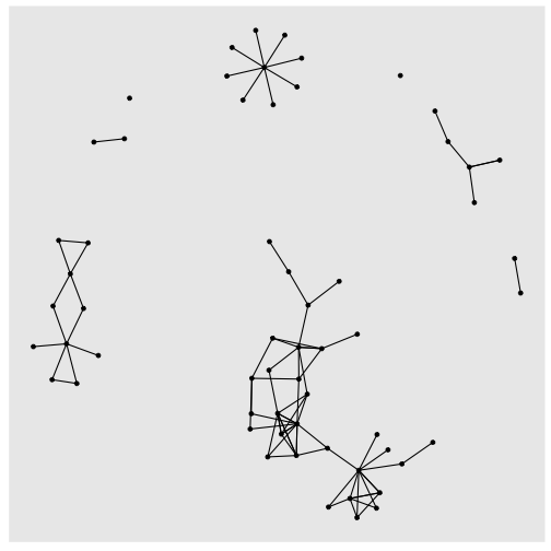
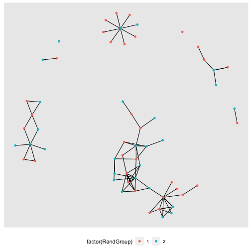
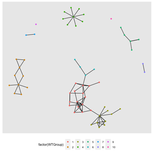
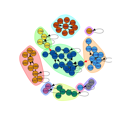
class: center, middle, inverse, title-slide .title[ # PEER Advanced Field School 2023 ] .subtitle[ ## Day 3 - Whole Networks ] .author[ ### Eric Brewe <br> Professor of Physics at Drexel University <br> ] .date[ ### 15 June 2023, last update: 2023-06-22 ] --- # Welcome Back! ### Our project is about building and analyzing the Workshop network We will continue to use the data file from yesterday, WorkshopNetwork.rds. ```r library(tidyverse) #tools for cleaning data library(igraph) #package for doing network analysis library(tidygraph) #tools for doing tidy networks library(here) #tools for project-based workflow library(ggraph) #plotting tools for networks library(boot) #to do resampling ``` --- # Let's load our data ```r gr <- readRDS(here("data", "WorkshopNetwork.rds")) ``` --- # Let's plot it quickly While we are at it we might as well set a layout. .pull-left[ ## Whare are distinctive features of the network? ```` ```r GrLayout <- create_layout(gr, layout = "kk") ggraph(GrLayout) + geom_edge_link() + geom_node_point() + theme(legend.position="bottom") ``` ```` ] .pull-right[ <!-- --> ] --- # Let's explore whole network metrics **These are fairly easy to calculate** - Density: Proportion of possible connections that exist - Diameter: Longest Shortest Path across network - Reciprocity: Extent to which each directed edge is a two way edge - Transitivity: Extent to which three connected nodes form triangles - Average Path Length: Average shortest distance between every pair of nodes **These require a bit more work** - Giant: Number of nodes connected to largest component - Homophily: Extent to which nodes with similar attribute are connected - Average degree: This is pretty descriptive. This is a list of many common graph metrics used in tidygraph https://rdrr.io/cran/tidygraph/man/graph_measures.html --- # Lets calculate a couple of these... ### For many of these it is a very simple one line command. Here is density ```r edge_density(gr) ``` ``` ## [1] 0.02853107 ``` Here is diameter, note that with tidygraph you have to use the with_graph() function, and specify the graph and function graph_diameter() ```r with_graph(gr, graph_diameter()) ``` ``` ## [1] 6 ``` -- .center.font200[So?] --- # Let's calculate a couple of others ### It is your turn, choose one of the ones that are easy to calculate and make the calculation. -- ```r with_graph(gr, graph_reciprocity()) #Reciprocity ``` ``` ## [1] 0.2142857 ``` ```r transitivity(gr) #Transitivity ``` ``` ## [1] 0.2669492 ``` ```r with_graph(gr, graph_mean_dist()) #Average Distance ``` ``` ## [1] 1.88125 ``` --- # Let's create a function ### Creating a function accomplishes two things: 1. We can calculate some of the harder to calcluate metrics 2. We do not have to re-do each time we want to analyze a new network. ```r GrFunction <- function(gr){ Giant = max(clusters(gr)$csize) AveDeg = gr %>% activate(nodes) %>% mutate(Deg = centrality_degree( mode = 'total') ) %>% select(Deg) %>% as_tibble() %>% summarise(AveDeg = mean(Deg)) df = tibble(Giant, AveDeg ) return(df) } ``` --- # Let's run this function ```r GrFunction(gr) ``` ``` ## # A tibble: 1 × 2 ## Giant AveDeg ## <dbl> <dbl> ## 1 30 3.37 ``` ### What do these numbers mean? -- *Giant* = 30, there are 30 people connected in the largest component. *AveDeg*, the average person has 3.37 incoming or outgoing edges --- # Let's talk about clustering Whole networks sometimes have regions which are different. Perhaps you want to know, are there groups that have some common characteristic? So we need a way to look for groups within our network. ### Start with random assignment: ```` ```r #First generate a grouping based on random assignment. gr %>% activate(nodes) %>% mutate(RandGroup = sample(1:2,60, replace = TRUE)) -> gr ``` ```` --- # Let's plot this with the random assignment to groups .pull-left[ ```` ```r GrLayout <- create_layout(gr, layout = "kk") ggraph(GrLayout) + geom_edge_link() + * geom_node_point(aes(color = factor(RandGroup))) + theme(legend.position="bottom") ``` ```` ] .pull-right[ <!-- --> ] --- # Let's talk about Modularity Modularity is a metric that tells us whether there is a way to break up our network into chunks which have more connections within the chunk than from the chunk to other parts of the network. ```r with_graph(gr, graph_modularity(group = RandGroup)) #Modularity ``` ``` ## [1] 0.01470444 ``` So the modularity of our network with nodes randomly assigned to groups is .12 This means that based on our grouping, there is a very slightly greater proportion of links between members of the group than across groups. --- # Let's use an actual community detection algorithm We'll use Walktrap, in which a random surfer can jump node to node based on the presence of edges. Then the walktrap algorithm establishes community structure by finding the propensity to end up in a cluster of nodes. There are two ways to do this... ```r #First generate a grouping based on the walktrap algorithm and add it to the graph. gr %>% activate(nodes) %>% mutate(WTGroup = group_walktrap()) -> gr #The other way is to just call the walktrap algorithm. wtg <- with_graph(gr, group_walktrap()) wtg ``` ``` ## [1] 9 3 5 1 2 7 2 4 1 1 4 3 1 5 6 3 8 2 10 1 1 4 5 3 2 ## [26] 4 4 6 1 4 4 4 1 7 3 2 2 2 2 2 4 1 1 1 1 1 3 3 3 3 ## [51] 3 1 1 5 5 6 6 8 2 1 ``` --- # Let's talk about Modularity Now we can check the modularity with the walktrap defined communities ```r with_graph(gr, graph_modularity(group = WTGroup)) #Modularity ``` ``` ## [1] 0.7393393 ``` So the modularity of our network with nodes assigned to groups via the walktrap algorithm is .74 This means that based on our grouping, there is a much greater proportion of links between members of the group than across groups. --- # Let's plot the walktrap communities This is the hard way to plot these. .pull-left[ ```` ```r GrLayout <- create_layout(gr, layout = "kk") ggraph(GrLayout) + geom_edge_link() + * geom_node_point(aes(color = factor(WTGroup))) + theme(legend.position="bottom") ``` ```` ] .pull-right[ <!-- --> ] --- # Let's plot the walktrap communities again This is the easy way to plot these (though not tidy). .pull-left[ ```` ```r wtg = cluster_walktrap(gr) modularity(wtg) plot(wtg, gr) ``` ```` ] .pull-right[ ``` ## [1] 0.6267523 ``` <!-- --> ] --- # Now it is your turn - Choose a community detection algorithm, - calculate it for the Workshop Network, and - be ready to talk about what the salient points of the community detection algorithm you chose. Here are the community detection algorithms available to you in tidygraph. https://tidygraph.data-imaginist.com/reference/index.html#community-detection